Dyno and Dyno Lab: Macroeconomic Models on Notebook.link

Writing, solving and simulating economic models in the browser
The models used in macroeconomics are often small: a dozen equations and a few parameters. Running them is another matter. The standard tool, Dynare, is excellent, but it requires MATLAB or Octave and a preprocessor compiled for your platform. When I teach, getting this installed on every student's laptop often takes up most of the first session.
Dyno started as a way to solve these models with plain Python. Working with QuantStack as a scientific advisor, I have followed the progress of JupyterLite and emscripten-forge closely, and with Notebook.link Dyno can now be used without installing anything at all. The demo below opens a JupyterLab session with Dyno, its model editor and a set of example notebooks. All the computations run in your browser.
👉 Open the interactive demo or watch the video presentation:
What is Dyno?
Dyno is a Python library to specify, solve and simulate dynamic macroeconomic models (DSGE, RBC, New Keynesian), the kind of models used at central banks and in graduate macro courses. Models are written in a small language with explicit time indices:
α <- 0.36
β <- 0.99
δ <- 0.025
ρ <- 0.95
γ <- 2.0

z[~] <- 0.0
k[~] <- ((1/β - (1-δ)) / α)**(1 / (α-1))
y[~] <- k[~]^α
i[~] <- δ * k[~]
c[~] <- y[~] - i[~]

z[t] = ρ * z[t-1] + e_z[t]
y[t] = exp(z[t]) * k[t-1]^α
k[t] = (1-δ) * k[t-1] + i[t]
c[t] = y[t] - i[t]
β * (c[t+1]/c[t])^(-γ) * (α * y[t+1]/k[t] + 1 - δ) = 1

e_z[t] <- N(0.01)
[t-1], [t] and [t+1] refer to the previous, current and next period, and
[~] to the steady state. Dyno checks the steady state and the
Blanchard-Kahn conditions, solves the model by perturbation, and computes
impulse responses, moments and simulations. It can also generate a report
describing the model. Deterministic (perfect foresight) models are solved with
a stacked-time Newton method. There is preliminary support for Dynare .mod
files, so that existing models can be reused.
The library itself is written in Python and depends on NumPy, SciPy, pandas and Altair.
Dyno Lab
Most of the work on a model consists in editing it: changing a calibration,
adding an equation, finding a wrong sign. Dyno Lab (jupyterlab-dyno) is a
JupyterLab extension meant for this.
When you open a .dyno or .mod file, a preview panel opens next to the
editor. Each time the file changes, the model is parsed and solved again, and
the preview shows the steady-state check, the eigenvalues, the decision rules
and the impulse responses.
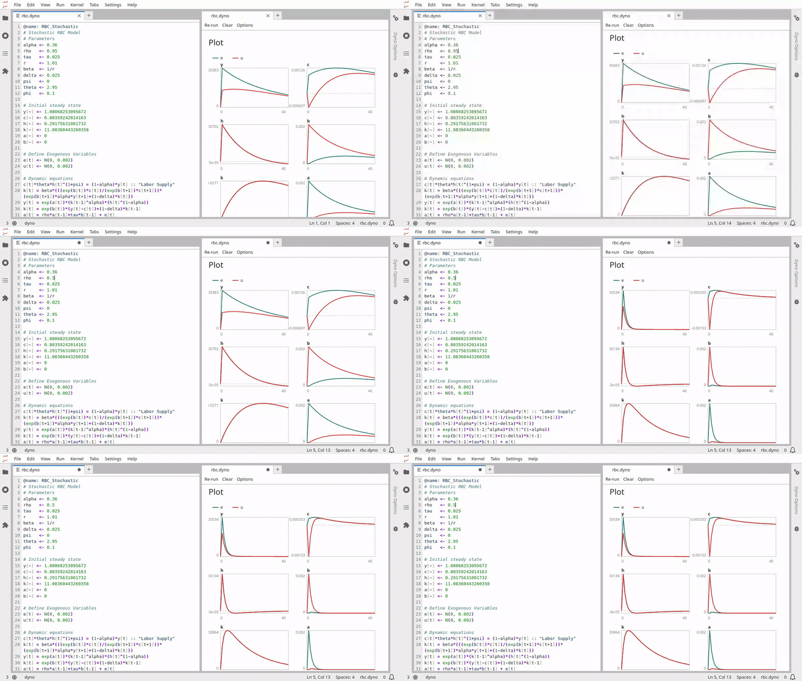
Editing an RBC model in Dyno Lab.
Errors are highlighted in the editor at the line where they occur. The model
file can also list what should be computed and plotted, using @run:
directives (check, solve, simulate, plot).
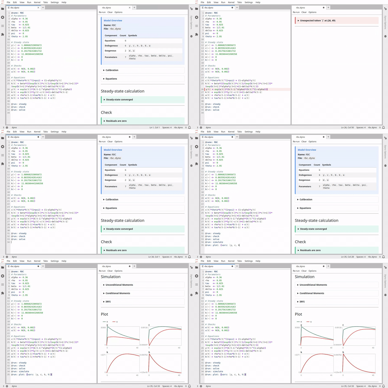
Error highlighting and @run: directives in Dyno Lab.
How it runs in the browser
In the demo, there is no server doing the computations. When you open the link:
- the Python kernel runs in the browser, compiled to WebAssembly;
- NumPy, SciPy and pandas are the WebAssembly builds from emscripten-forge;
- Dyno and Dyno Lab are pure Python (
noarch) conda packages from theeconforgechannel, the same ones you get withpixi add dyno jupyterlab-dynoon your own machine; - the environment is described by an environment file in the demo repository, which Notebook.link reads to build it.
For us, this is the most useful aspect. We did not have to write a separate web version of Dyno. The extension communicates with the kernel through the usual Jupyter messages, and it works in the same way with a local Python process or with a WebAssembly kernel. Once the packages were published, getting them to run on Notebook.link mostly amounted to writing an environment file.
What is in the demo
The demo contains four notebooks. They are written so that someone without a background in economics can follow them, while still being of interest to Dynare users.
- Getting started. A real business cycle model: we solve it, plot impulse responses to a technology shock and simulations, and compare calibrations. Economic terms are defined when they first appear.
- Deterministic models. Transition paths after an anticipated productivity increase, or after a large destruction of capital, computed with the nonlinear perfect-foresight solver.
- Dynare compatibility. The same model written as a
.modfile and as a.dynofile, solved both ways, with the results compared. - Reports and pipeline. Producing a report from a model file.
There is also a file named double_click_me.dyno. It is a short tutorial in
which you build a model of inflation step by step, by un-commenting lines one
at a time and looking at how the preview changes. If you only have a few
minutes, start there.
Uses in teaching and research
In a course, a link on a slide or in a problem set is enough for students to start working on a model, whatever computer they have. Because the computations run on each student's machine and not on a server, the number of users is not a concern: a class of two hundred students opening the link at the same time needs no more infrastructure than a single reader, and there is no JupyterHub to set up or pay for.
Reproducibility is the other benefit. The environment is managed by mamba from standard conda packages, with versions pinned in the repository's environment file, so everyone who opens the link gets the same versions of Dyno and its dependencies. The same packages can be installed on a laptop with conda, mamba or pixi. For research, a link to a notebook lets a referee or a reader change a parameter in a published model and look at the result, in an environment that can be rebuilt later.
What comes next
The main item on our roadmap is better compatibility with Dynare .mod files,
which we are working on together with the Dynare team. The current support
only covers part of the syntax. We also have a proof of concept in which the
Dynare preprocessor is compiled to WebAssembly and runs in the browser, which
would eventually allow .mod files to be handled by the same code as in
Dynare.
We are also working on higher-order perturbation and on more examples for teaching. If you teach macro and would like to publish course material on Notebook.link, feel free to get in touch.
- Demo: notebook.link/github/EconForge/dyno-short-demo
- Video: YouTube
- Dyno: EconForge/dyno.py (documentation)
- Dyno Lab: EconForge/jupyterlab-dyno
Acknowledgements
Selma Malmberg contributed an early implementation of the solver. As an intern, Ousema Bouaneni built the proofs of concept for both the interactive JupyterLite interface and a Python binding of the Dynare preprocessor. Thanks to Sébastien Villemot from the Dynare team for helping us compile the Dynare preprocessor. Finally, this work would not run in the browser without the JupyterLite, emscripten-forge and Notebook.link work of the QuantStack team, with whom it has been a pleasure to collaborate.